SciPy
SciPy is a Python-based ecosystem of open-source software for mathematics, science, and engineering.
SciPy is organized into sub-packages that cover different scientific computing domains. In this SciPy Tutorial, we shall learn all the modules and the routines/algorithms they provide.
SciPy contains following modules :
- Cluster
- Constants
- FFTpack
- Interpolate
- Input and Output
- Linalg
- Ndimage
- Optimize
- Stats
- CSGraph
- Spatial
- ODR
- Special
SciPy Tutorial
In this SciPy tutorial, we will go through each of these modules with necessary examples to understand SciPy Basics.
SciPy Cluster Module
Clustering is the process of organizing objects into groups whose members are similar in some way.
K-Means
SciPy K-Means : Package scipy.cluster.vp provides kmeans() function to perform k-means on a set of observation vectors forming k clusters.
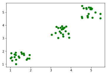
In this example, we shall generate a set of random 2-D points, centered around 3 centroids.
scipy-example.py
# import numpy
from numpy import vstack,array
from numpy.random import rand

# matplotlib
import matplotlib.pyplot as plt

# scipy
from scipy.cluster.vq import kmeans,vq,whiten

data = vstack(((rand(20,2)+1),(rand(20,2)+3),(rand(20,2)+4.5)))

plt.plot(data[:,0],data[:,1],'go')
plt.show()
Try Online
scipy-example.py
# whiten the features
data = whiten(data)
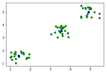
# find 3 clusters in the data
centroids,distortion = kmeans(data,3)
print('centroids : ',centroids)
print('distortion :',distortion)
plt.plot(data[:,0],data[:,1],'go',centroids[:,0],centroids[:,1],'bs')
plt.show() Try Online Output
centroids  :  [[ 1.42125469  1.58213817]
 [ 3.55399219  3.53655637]
 [ 4.91171555  5.02202473]]
distortion : 0.35623898893
Constants
SciPy contains physical and mathematical constants and units. Following list provides the broad categories and some of the examples.
- Mathematical Constants
- Physical Constants
- SI Prefixes(kilo, mega, zeta)
- Binary Prefixes(kibi, mebi, zebi)
- Angle: degree, arcsec, etc., in radians
- Time: minute, hour, week in seconds
- Length: mile, yard, micron, etc., in meters
- Pressure: atmosphere, torr, psi, etc., in Pascals
- Area: hectare, acre in square meters
- Volume
- Speed
- Temperature
- Energy
- Power
- Force
- Optics
FFTpack
FFT
scipy.fftpack provides fft function to calculate Discrete Fourier Transform on an array.
fft-example.py
# import numpy
import numpy as np

# import fft
from scipy.fftpack import fft

# numpy array
x = np.array([1.0, 2.0, 1.0, 2.0, -1.0])
print("x            : ",x)

# apply fft function on array
y = fft(x)
print("fft(x)       : ",y)
Try Online Output
x : [ 1. 2. 1. 2. -1.]
fft(x) : [ 5.00000000+0.j -1.11803399-2.2653843j 1.11803399-2.71441227j
  1.11803399+2.71441227j -1.11803399+2.2653843j ]
IFFT
scipy.fftpack provides ifft function to calculate Inverse Discrete Fourier Transform on an array.
ifft-example.py
# import numpy
import numpy as np

# import fft
from scipy.fftpack import fft, ifft

# numpy array
x = np.array([1.0, 2.0, 1.0, 2.0, -1.0])
print("x            : ",x)

# apply fft function on array
y = fft(x)
print("fft(x)       : ",y)

# ifft (y)
z = ifft(y)
print("ifft(fft(x)) : ",z)
Try Online Output
x : [ 1. 2. 1. 2. -1.]
fft(x) : [ 5.00000000+0.j -1.11803399-2.2653843j 1.11803399-2.71441227j
  1.11803399+2.71441227j -1.11803399+2.2653843j ]
ifft(fft(x)) : [ 1.+0.j 2.+0.j 1.+0.j 2.+0.j -1.+0.j]
Integrate
scipy.integrate contains many functions to compute definite integral.
In this example we will compute a definite integral using scipy.integrate.quad() function.
>>> from scipy import integrate
>>> x2 = lambda x: x**2
>>> integrate.quad(x2, 0, 4)
(21.333333333333332, 2.3684757858670003e-13)
Try Online
In the first line, we imported integrate module from scipy package. Then we created a lambda function x2 which is the square of input variable. We then passed this function to the quad() function with lower limit as 0 and upper limit as 4.
In the output of quad() function, the first value is the approximate value of the integral and the second value is an estimate of absolute error.
Interpolate
Interpolation is the process of finding the function, given input and output values. Interpolation is used regularly, where we have an experimental data containing inputs and outputs, and estimate the output for new inputs.
SciPy provides a variety of interpolate functions. In this example, we will take an equation y = f(x). Consider that we have performed a set of experiments and we have x values and their corresponding y values.
>>> import numpy as np
>>> from scipy import interpolate
>>> x = np.arange(0, 10)
>>> y = np.exp(-x/3.0)
>>> f = interpolate.interp1d(x, y)
>>> x
array([0, 1, 2, 3, 4, 5, 6, 7, 8, 9])
>>> y
array([1.        , 0.71653131, 0.51341712, 0.36787944, 0.26359714,
       0.1888756 , 0.13533528, 0.09697197, 0.06948345, 0.04978707])
>>> f(0.5)
array(0.85826566)
>>> f(1.5)
array(0.61497421)
>>>
Try Online interp1d() returns a lambda function and is stored in f. Now you can estimate y values for new x values. We have estimated y values for x=0.5 and x=1.5.